A Comprehensive Guide to Testing iOS GPS Accuracy

Jun 3, 2019 • Trevor Phillips

Hundredths of a second typically separate Gold medalists and Silver medalists in an Olympic track race, and as such, precise timing measurements are critical.

Even if you’re not training for the next Olympic Games, you probably want an accurate estimate of distance and time when you go for a run. At Freeletics, we strive to make our app as precise as possible when our users do running workouts.

What follows is an exploration of how we determined the accuracy of raw data from an iPhone GPS sensor, how we built a framework to improve this accuracy, and how we systematically validated these improvements compared to raw data.

Background

CLLocation

In the realm of iOS development, an app receives GPS locations by subscribing to updates from a CLLocationManager. Each GPS location received is called a CLLocation and has the following properties:

• coordinate: Latitude and longitude in degrees
• altitude: A value given in meters above/below sea level
• horizontalAccuracy: A radius of uncertainty around the coordinate, given in meters. A higher value corresponds to less accuracy.
• verticalAccuracy: A range of uncertainty centered at altitude. A higher value corresponds to less accuracy.
• course: The direction of travel, measured in degrees relative to due north and continuing clockwise around the compass
• speed: The user’s speed in meters per second
• timestamp: An object containing the specific date and time that the location was measured

The Game Plan

Our approach in improving the accuracy of GPS data was to…

1. Collect CLLocation data in various conditions (sunny, cloudy, city, park, etc.)
2. Determine typical values for the aforementioned CLLocation properties and the levels of “noise” for these properties
3. Generate a true path (the path the user actually ran) and a noisy path (simulating raw GPS data) for combinations of various conditions
4. Build a function which takes the noisy path as input and outputs an estimate of the true path–we will call this output the estimated path
5. Validate the function by verifying that the total distance of the estimated path is closer to the total distance of the true path than that of the noisy path

1. Data Collection

To collect raw GPS data, we created a special version of our app for use by employees only. With this special version, the sequence of CLLocation objects received from the GPS sensor during a run is sent to the developer team after the user has finished his or her workout.

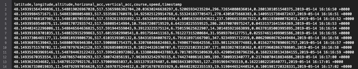GPS data of a CLLocation sequence, represented in CSV format

This data can be thought of as the “noisy path.” When an employee would submit GPS data, we would then ask him to draw the exact “true path” that he ran and take note of the environmental conditions during the run.

We used onthegomap.com for marking the true path, which allows one to download a GPX file containing a sequence of coordinates. The GPX file is converted into a CSV format similar to that of the raw data using this Python script.

Unfortunately onthegomap.com lacks elevation data, but we programmatically inserted altitude information using Google’s Elevation API based on each location’s latitude and longitude.

2. Data Analysis

Armed with a rich dataset of CLLocation sequences, we are ready to begin analysis. The parameters we care about are the mean and standard deviation of:

• The separation in meters between two consecutive locations
• The time in seconds between two consecutive location measurements
• The horizontalAccuracy property
• The verticalAccuracy property

We want the mean and standard deviation to generate a realistic “noisy path” based on a given “true path.” An important assumption moving forward is that these four attributes will follow normal distributions, i.e., that measurements will be centered around the mean with some variability which decreases in likelihood as we move away from the mean.

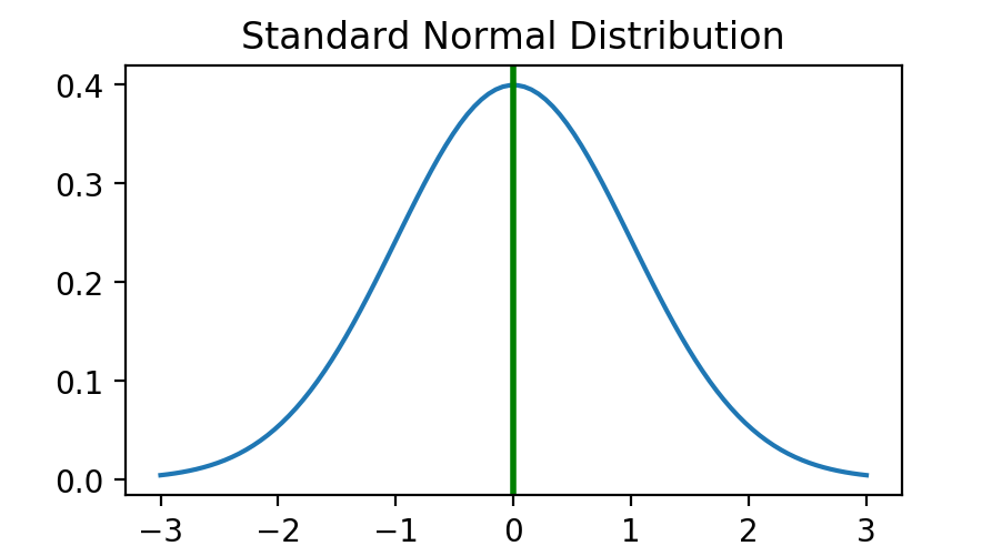Standard normal distribution has mean=0.0 and standard deviation=1.0

Initial Insights

• The mean distance between consecutive locations was 0.952 meters
• The mean time between consecutive measurements was 1.000 seconds and the standard deviation was 0.131 seconds
• horizontalAccuracy varied depending on environmental conditions, but the overall average was 7.179 meters with a standard deviation of 1.682 meters
• verticalAccuracy also varied depending on conditions, but the average was 3.643 meters with standard deviation of 0.300 meters
• The accuracy is much worse for the first 10–20 measurements and then stabilizes after that

The error rate of raw GPS data compared to the “true path” of the user was quite good in some cases–within 0.28% of the true distance–but in other cases as much as 7% off from the actual distance covered by the user.

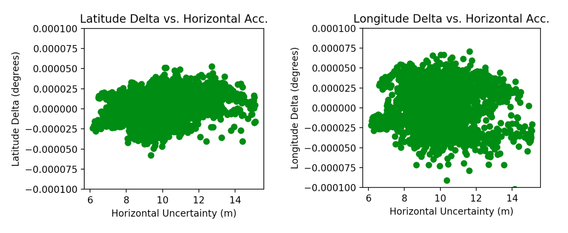
We might expect a correlation between the level of inaccuracy and the distance between consecutive points. In other words, a tendency for more “jumping around sporadically” when the accuracy is low. However, plotting the relationship between these two variables does not reveal a trend. This suggests that Apple may already be performing some rudimentary filtering of raw GPS data.

3. Simulating “True” and “Noisy” Paths

Remember, the goal is to build a function which takes noisy data as input and will output an estimate of the true path. We’re going to define this function in the next section, but to ensure that it will work correctly, we need to test it in a variety of scenarios. Each scenario is generated using the statistics we calculated in the previous section.

We define a scenario as the following Swift struct:

Furthermore, we define the following enums as potential environmental conditions which affect a scenario:

We create a scenario for each possible combination of conditions, which works out to 2 × 3 × 3 × 3 = 54 scenarios.

True Path of a Scenario

To create a scenario given some set of parameters (pathType, distance, speed, signalStrength), first we build the “true path” as an array of CLLocation objects. If the pathType is loop, we build the true path as a perfect circle around an arbitrary center point where the circumference of the circle is equal to the distance attribute. If the pathType is outAndBack, the path simulates a user running straight, turning right, running some more, and then going back the same way he came (again with the total distance equal to the distance attribute).

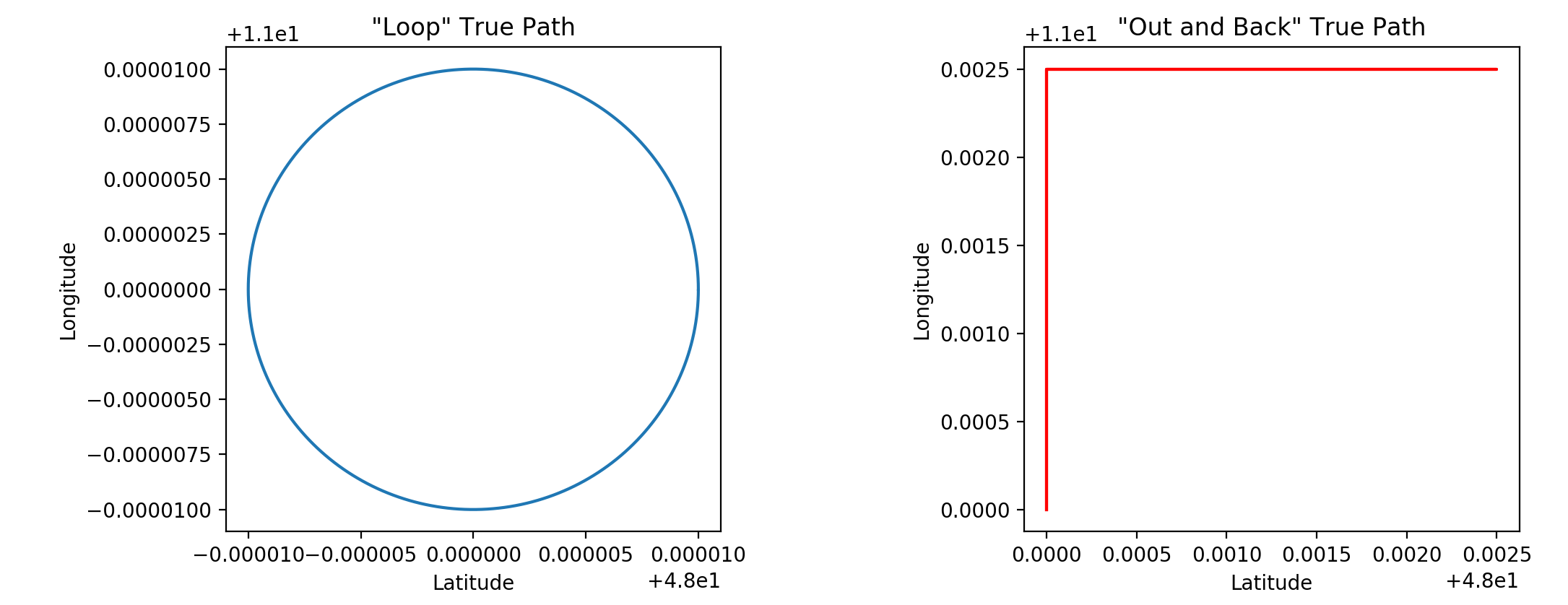
The speed parameter affects the “step size” between points on the true path. In other words, the greater the speed, the greater the distance between consecutive points on the path.

For the true path, we assume perfect accuracy such that horizontalAccuracy = 0 and verticalAccuracy = 0. We maintain an altitude of 0 meters and a time gap of 1 second between samples.

Noisy Path of a Scenario

For every true path in a scenario, we create a corresponding “noisy path” by adding noise to each CLLocation in the scenario’s truePath array. The noise is generated from a normal distribution using the means and standard deviations we determined in the previous section.

Below is a function to sample from a normal distribution with some given mean and standard deviation using the Box-Muller Transformation:

The rng variable is a GKRandomSource random number generator which is seeded with the value 100 for each scenario. We use a random number generator to keep everything deterministic and consistent when running tests.

To make things more concrete, here is an example of how one might convert a CLLocation from the true path into a CLLocation for the noisy path:

In the real implementation, the constants are stored in a separate file rather than hard-code into the conversion function as shown above

The signalStrength parameter affects which constants we use for the mean and standard deviation of the horizontalAccuracy and verticalAccuracy normal distributions. For example, the mean accuracy for a strong signal is smaller (more accurate) than that of a weak signal, and the standard deviation for a varied signal is greater (more variable) than that of a weak or strong signal.

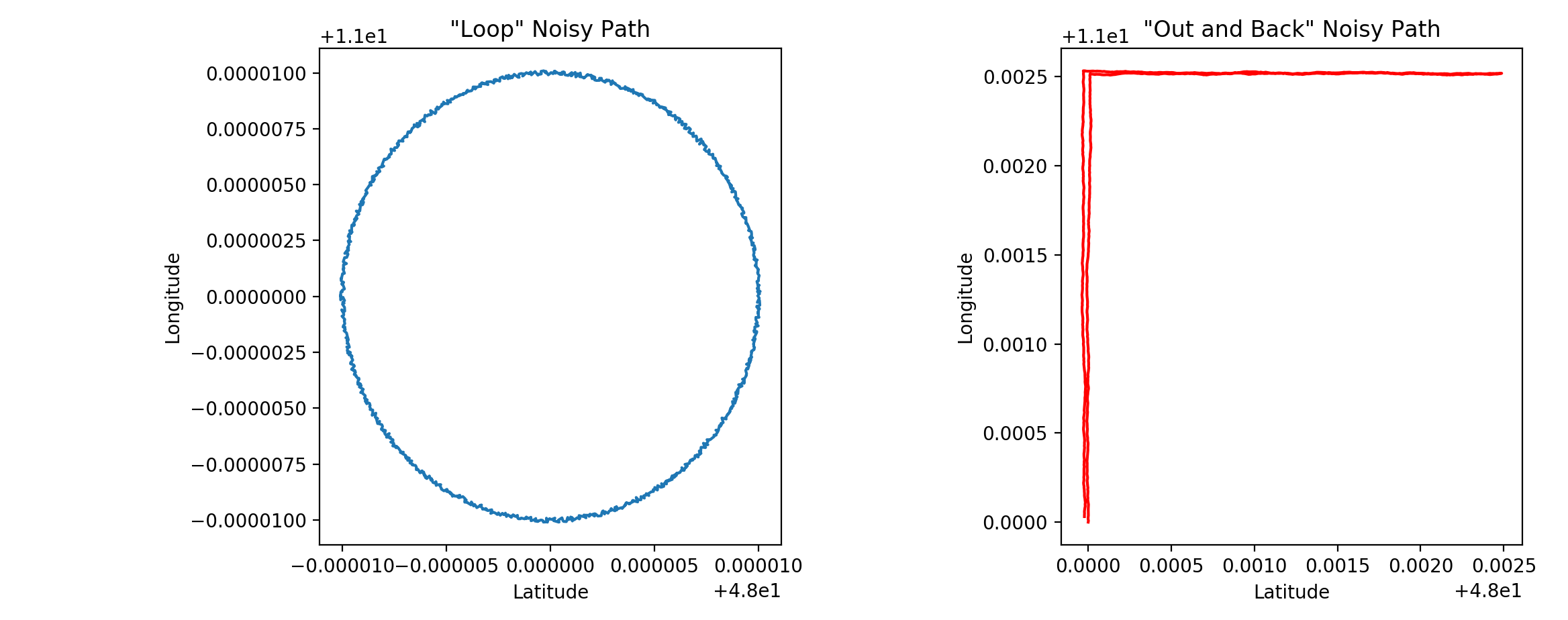Visualization of noise added to a “true path”

4. Filtering Noisy Data

Our goal is to build a function which takes a noisy path as input and outputs an estimated path which is as close to the true path as possible (without actually knowing the true path).

How? Enter… the Kalman filter

The Kalman filter is a mathematical construct used in many applications, from aircraft guidance to signal processing. Its usefulness lies in estimating the true value of a variable, given estimates of the variable over time.

Going into detail about Kalman filters is beyond the scope of this article, however Bzarg.com has an easy-to-follow post explaining the inner workings of the filter.

Below is an implementation adapted specifically for CLLocation:

With our Kalman filter ready to go, we can call

process(measurement: incomingLocation)

for each incoming “raw data point” received from CLLocationManager, thereby deriving a more accurate estimate of the user’s current location.

5. Validating the Kalman Filter

With the filter in place and a (truePath, noisyPath) pair for each of our 54 scenarios, we have everything needed for a comprehensive testing framework.

For each scenario, we perform the following check:

Results

We were able to achieve an accuracy level within 0.7% of the true distance in the best case, and within 1.68% in the worst case (depending on the distance of the GPS track and the simulated signal strength).

Moreover, we now have a general idea of the accuracy of raw GPS data and are able to systematically validate the performance of the Kalman filter.